💻 Final project: making a visualization of your own data
We would like you to spend the remainder of your time in this course on doing this little project. We have two options for you to choose from. The first and recommended one is making a visualization of your own (research) data. The second option is that you work on a visualization of data we have prepared.
Do not forget that if you are stuck to join us on Discord or in a feedback webinar so we can help. See the Course overview for more information.
If you made a nice visualization and still have time left in the course, why not make an animation?
Option 1: your own data
So far you have learned how to make meshes and vertex colors in Blender using Python. So, think about if you can visualize your data using these techniques. You need to think about what you need to do to transform your data into a form that can be used to generate vertices, faces and vertex colors. And how do you want to visualize your data values? Can you visualize them through the Cartesian coordinates of the vertices and faces and maybe some colors? Do you need to use vertex coloring? Or do you need something else? Note that volumetric data will be difficult in Blender and you may need to think of some tricks.
Option 2: visualize a computer model of a proto-planetary disk
Although we highly recommend you to work on your own data, if you have none to use, you can use the following data to work on. Here we give a brief introduction to the data.
What is a proto-planetary disk
A proto-planetary disk is a disk-like structure around a newly born star. This disk is filled with dust (solid-state particles with a diameter in the order of 1 micrometer) and gas. In the course of time this dust and gas can coalesce into planets. In this option we will look at a computer model of the dust in such a disk. The model calculates the temperature and density of the dust in the disk, taking the radiation and gravity of the star into account.
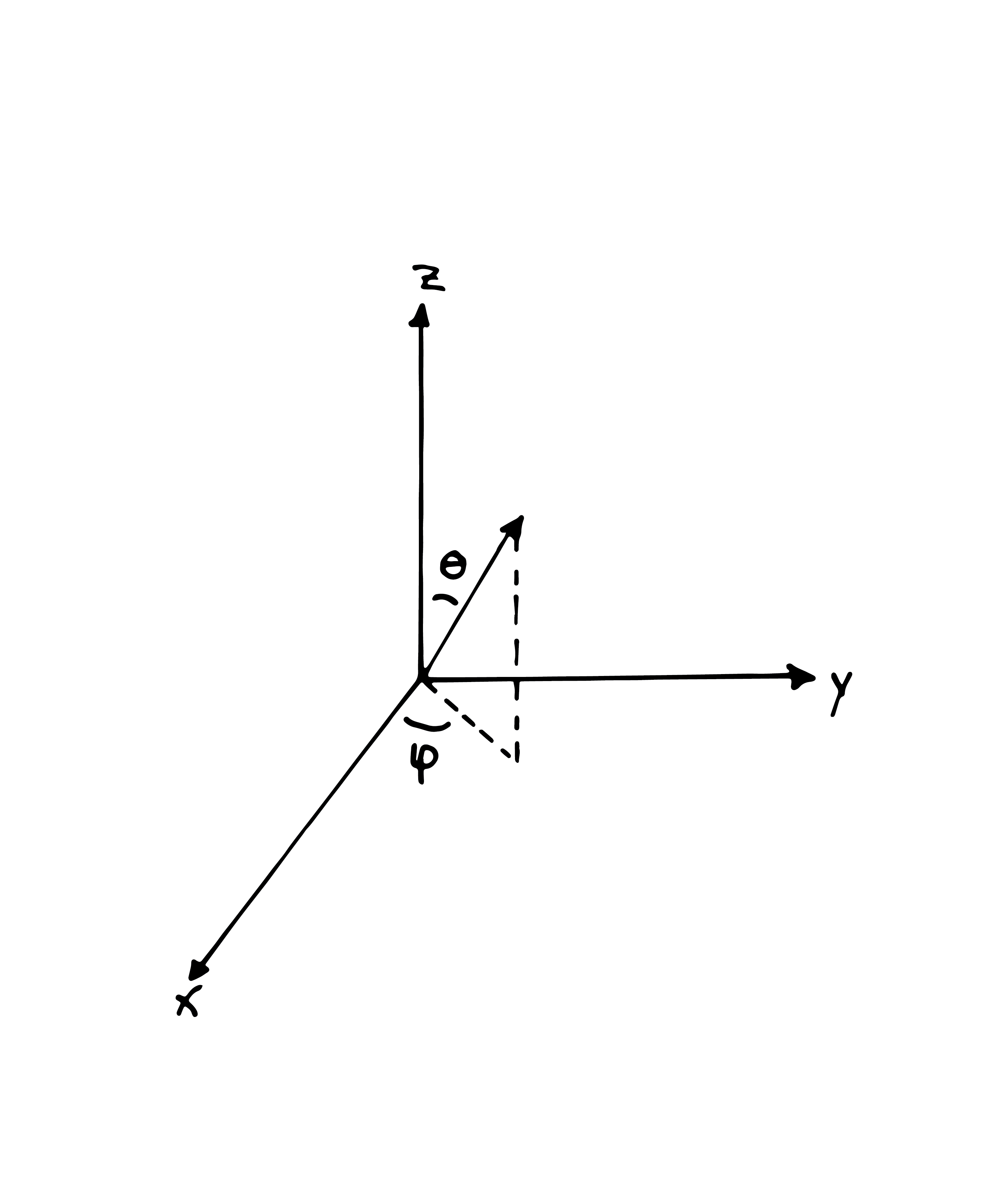
The calculations of the software (called MCMax) are done iteratively using Monte Carlo techniques. Packages of photons are emitted by the star in random directions and their wavelength sampled from the radiation distribution of the star (by default a blackbody). Using the absorption, scattering and emission properties of the dust grains in the disk, the scattering, absorption and re-emission of the photons are calculated throughout the disk. This is used to calculate a temperature structure in the disk. This temperature is then used to adapt the starting density structure of the disk after which a new pass is done by tracking a next set of photons and adapting the density subsequently. This is repeated until convergence is reached. The code uses a two dimensional (adaptable) grid in the radial and theta direction. The disk is assumed to be cylindrically symmetric around the polar axis (z-axis, see Fig. 1). The grid cell size is lowered in regions where the density becomes high.
How to start visualizing such a proto-planetary disk
You could create a 3D model of the disk at constant density and display the temperature as colors on the surface of the model. You could use this to make nice renders and animations to show the temperature structure of the disk. For this we need to pre-process the data from the model to get the spatial coordinates of the disk at a constant density. These coordinates then need to be converted into Cartesian coordinates of vertices and faces before creating the geometry in Blender. You can then add the temperatures to the faces using vertex coloring and by adding the needed shaders to the model.
How the model data is structured
You can download the data here. An example output file of modeling code MCMax is shown below.
# Format number
     5
# NR, NT, NGRAINS, NGRAINS2
   100   100     1     1
# Spherical radius grid [cm] (middle of cell)
   7479900216981.22
   7479900572789.07
[...]
# Theta grid [rad, from pole] (middle of cell)
  9.233559849414326E-003
  2.365344804038962E-002
[...]
# Density array (for ir=0,nr-1 do for it=0,nt-1 do ...)
  1.001753516582521E-050
  1.001753516582521E-050
[...]
# Temperature array (for ir=0,nr-1 do for it=0,nt-1 do ...)
   1933.54960366819
   1917.22966277529
[...]
# Composition array (for ir=0,nr-1 do for it=0,nt-1 do ...)
   1.00000000000000
   1.00000000000000
[...]
# Gas density array (for ir=0,nr-1 do for it=0,nt-1 do ...)
  1.001753516582521E-048
  1.001753516582521E-048
[...]
# Density0 array (for ir=0,nr-1 do for it=0,nt-1 do ...)
  1.001753516582521E-050
  1.001753516582521E-050
[...]
The data from the MCMax code is in spherical coordinates, while the system in Blender works with Cartesian coordinates. The theta in the output is defined as the angle with the z-axis (See Fig. 1).
How it could look
To help you get an idea of what the data of the proto-planetary disk might look like, check this video we made: