Introduction
Geometry Nodes are a way to program your own modifier that modifies your geometry, or generates new. Some predefined modifiers (like for example Subdivision or Decimate) in Blender were introduced in the section Simple Mesh Editing in the Basics part of the course. Modifiers can be added in the Modifiers tab in the Properties Editor (see Fig. 1). But how you will most likely be working with Geometry Nodes is through the Geometry Nodes Workspace, which can be found as a tab in the top part of the interface (see Fig. 1).
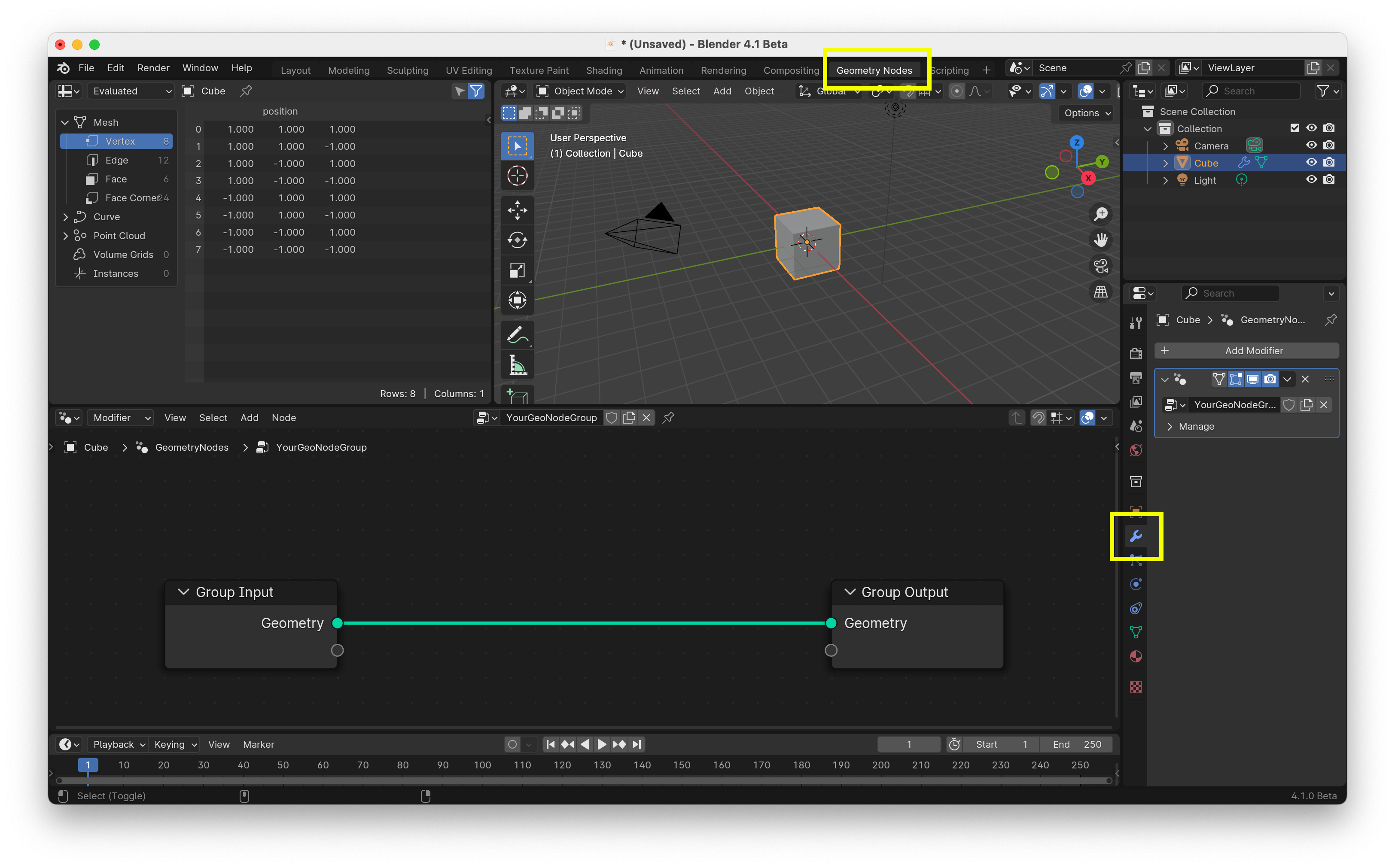
When you create a new Geometry Node Group you get a Group Input and a Group Output node, see Fig. 1. The geometry on which the geometry node modifier works is inputted through the Group Input node. And in Fig. 1 you see the Group Input node as an output 'Geometry' and this output has a circular, green, output socket. This output socket is connected to the input of the Group Output node. This node gives the output of the modifier and this is shown in the 3D view (passed to the next modifier if more are present on the object).
💻 Exercise 1
See what happends when you disconnect the two Group nodes in Fig. 1. Figure out how to reconnect the two Group nodes again.
Nodes & Connections
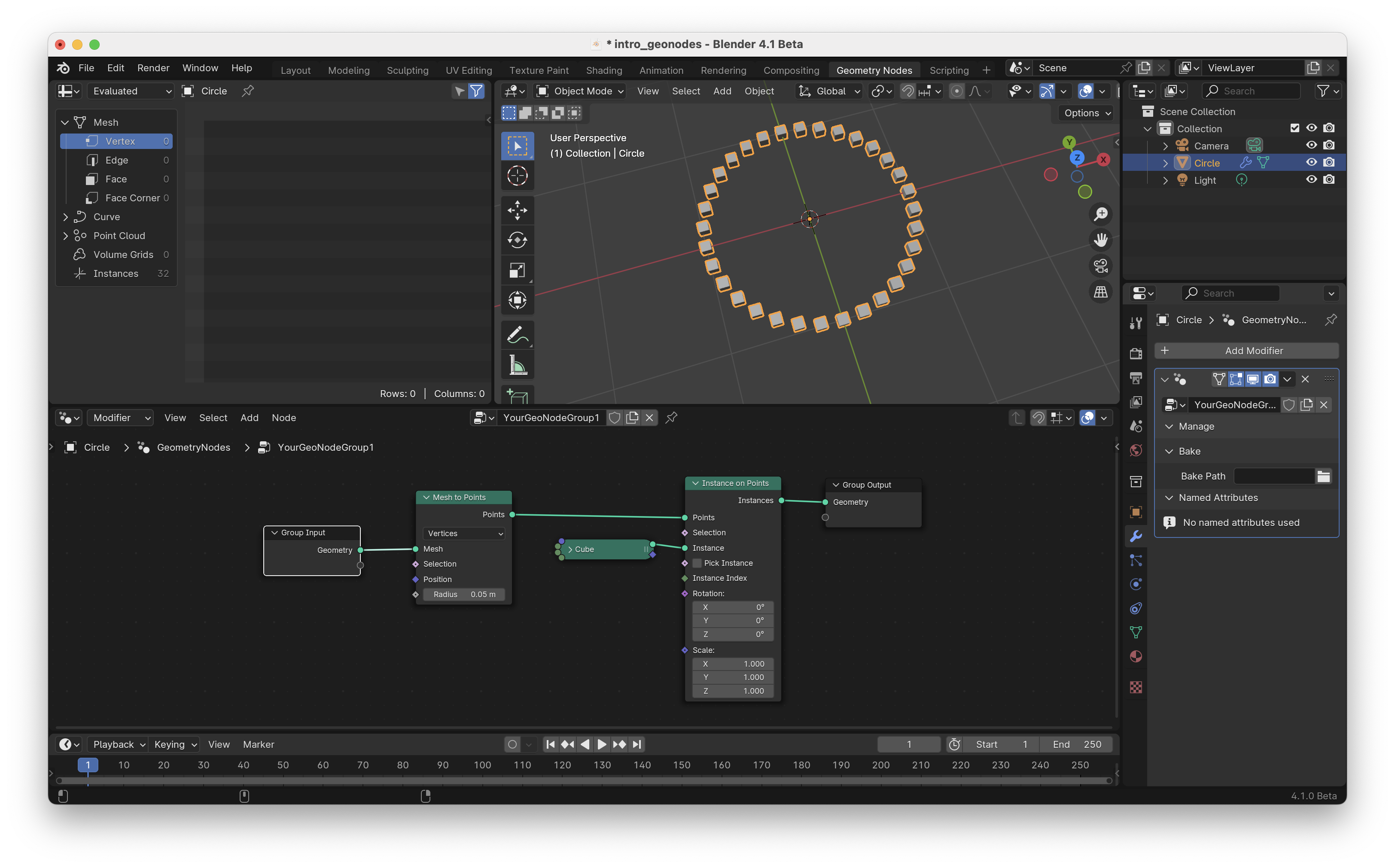
We will start with a simple example to see how Geometry Nodes work. In Fig. 2 we use a standard circle (in the 3d view type Shift-A and choose a circle from the Mesh menu) as the basis geometry on which we will create a Geometry Node modifier. The geometry on which the Geometry Node modifier is working comes with in through the Group Input node. We then create a point on every vertex using a Mesh to Points node. And then on every point we create a cube using the Instance on Points node which we tell to use a cube at every point by feeding it the Cube node. In the 3d view you can now see a whole bunch of cubes arranged on a circle.
Sockets & Fields
Lets do something more with the example in Fig. 2. Lets make it so that the cubes we make scale with their position on the x-axis. Fig. 3 shows how you can do this. We use the blue diamand shaped input socket named 'Scale' of the Instances on Points node. We connect this to a couple of nodes that retrieve the x-position of the cubes. We start with a Position node. This outputs a position vector which we split in x, y and z components using the Separate XYZ node. We take the x-component and scale it using a Math node set to multiply. We then combine the scaled x-component with a constant y and z component using the Combine XYZ node. This way we scale the the cubes based on their position on the x-axis.
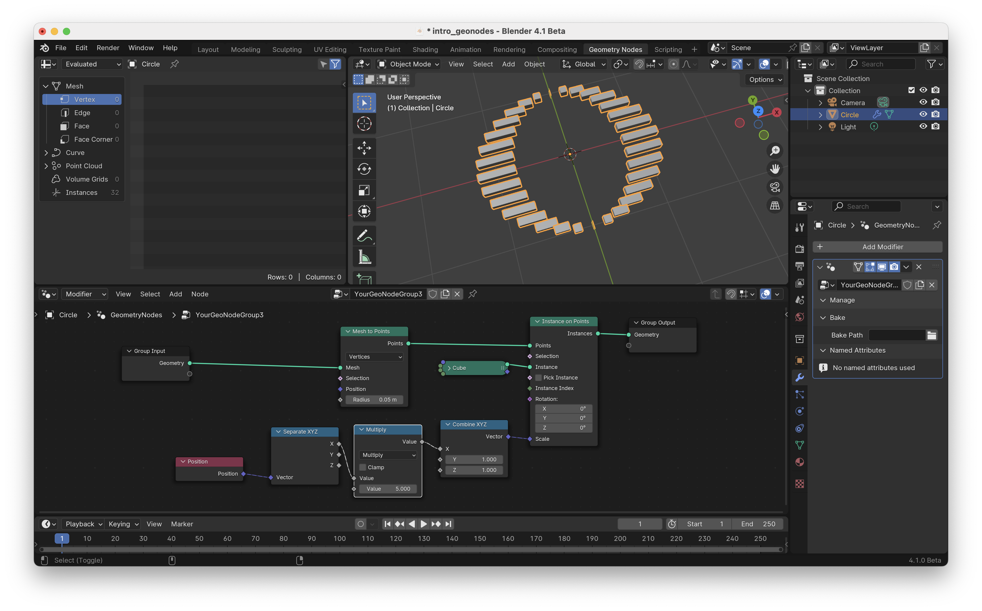
You can see that all the nodes building up to the 'Scale' socket, have dashed lines connecting diamond shaped sockets. This in contrast to the green solid lines with round sockets that are used for the flow of the geometry. The dashed lines are called fields and they are calculated differently from the solid lines. Field lines start with a node that generates data, in our example of Fig. 3 this is the Position node. These nodes need to know where to get the data from. What happens is that field lines are evaluated when they are connected to a node that has some geometry (solid line) fed into it. In our case this happens when the field is connected to the Instance on Points node. Now the Position node outputs the position of the points/vertices corresponding to the geometry that is connected to the Points socket in the Instance on Points. If you do not get this right away, do not worry. It is quite confusing at times, but it does allow for creating kind of functions as in programming languages.
To give an example of how fields work, lets connect some of the same nodes connected by field lines to another geometry. In Fig. 4 you can see I added a UV Sphere node that connects to a Delete Geometry node. Thus we create a sphere and now we want to delete part of the sphere using the 'Selection' socket of the Delete Geometry node. We will use the same Position node and Separate XYZ node as for the circle geometry, but now the position node will give the position of the vertices in the UV Sphere when I connect it to the Delete Geometry node. Here you see that you can connect the same Position node to different geometries and it will give different values. So you could also say that fields in Geometry Nodes are like functions that can be called by different nodes with different geometries.
💻 Exercise 2
Starting with a UV Sphere. Make an egg shaped object by elongating the UV sphere along, for example the x-axis. Tip: you could use a Set Position node and some of the nodes from Fig. 3 to do this.
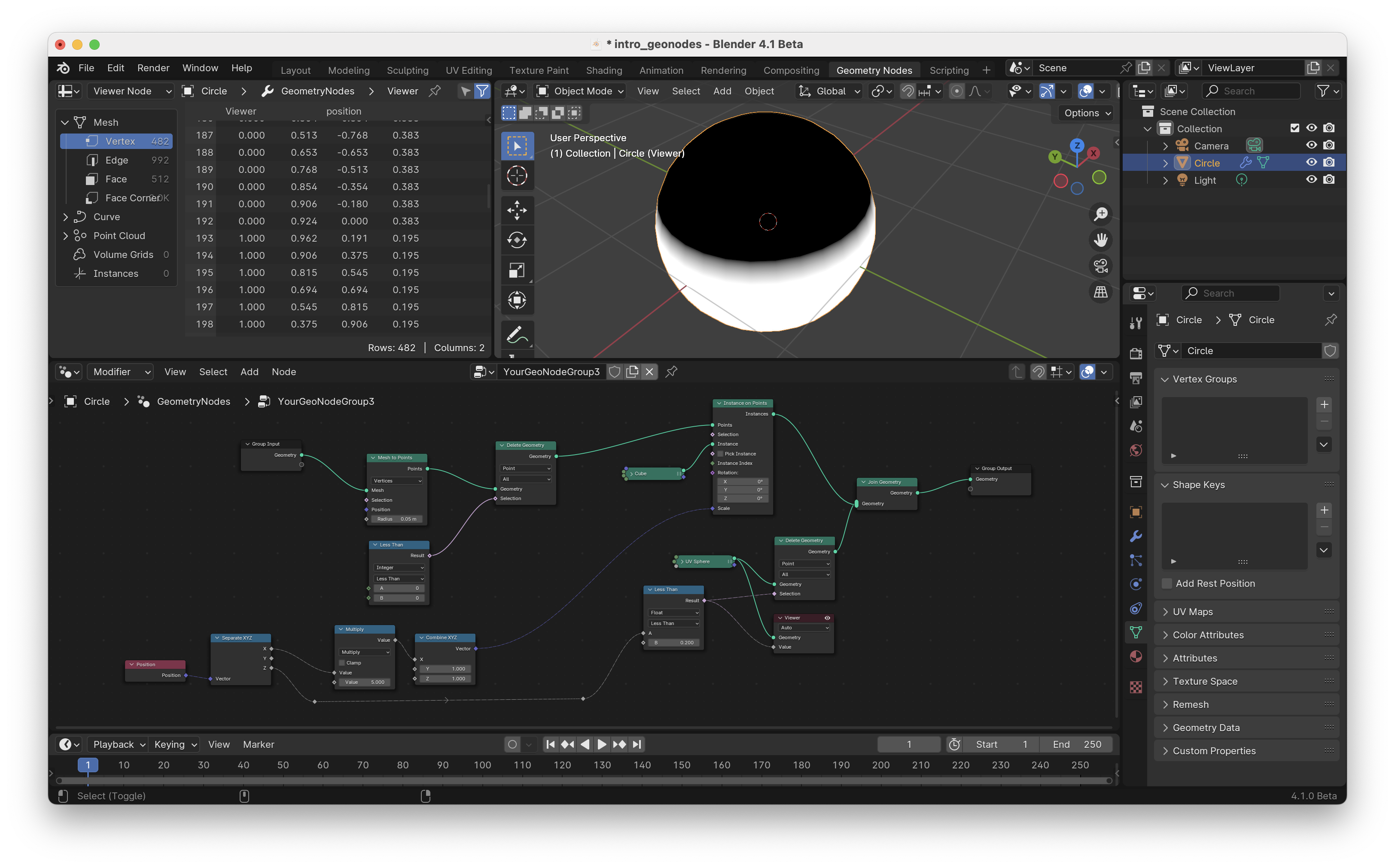
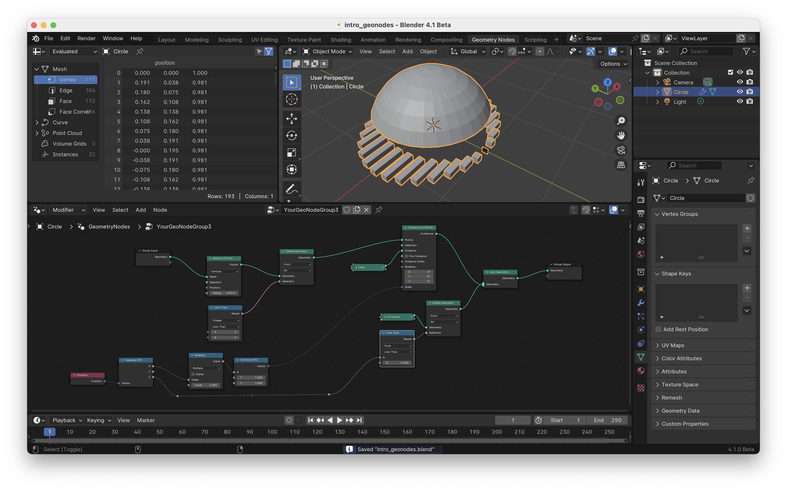
Viewer nodes
Before we start building more geometry nodes, let me quickly tell you about the Viewer node. This node is very useful for debugging and inspecting parts of your node tree. In Fig. 5 you can see I connected a viewer node directly to the UV Sphere node. When the little eye is visible in the top right of the viewer node, you can see its input in the 3D view. For example you now see the UV Sphere before part of its geometry is deleted. I also connected the boolean output of the Less Then Math node to the value socket of the viewer node. Doing this lets you inspect this value in the Spreadsheet editor (see top left of Fig. 5). Also it visualizes the value on the geometry in the 3D view, now you can see that the top half of the UV Sphere is black (representing false) and the bottom is white (representing true).